Chapter 16: Physiological Determinants of Athletic Performance

High jumping is a skill that requires a high degree of motor coordination, a high percentage of fast-twitch motor units in the leg muscles and physical height.

Case Study: Volunteer for a Research Study

Jake has volunteered to participate in a research project that requires him to complete an incremental test to exhaustion. He has done this before, so he is not apprehensive about the test. He follows the brief instructions prior to the test and shows up in the lab at the required time. Jake completes a 10 min warm-up of easy jogging, then sits for 10 min before beginning his test.

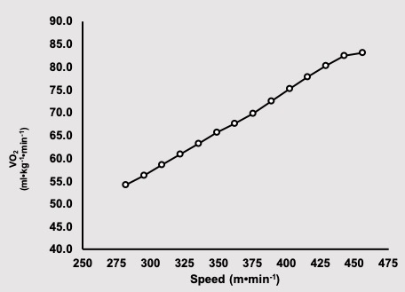
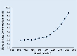
Preparation for the test included having a heart rate transmitter placed on Jake’s chest and a nose clip was put on his nose. He inserted the mouth piece into his mouth and took several breaths while the technician checked things out. Everything was working, so the test was initiated. Jake had been straddling the treadmill, so to begin running he simply supported his weight on his arms and started placing his feet on the moving treadmill belt. The speed of the treadmill was initially 281 m⋅s^-1, and the slope was 0%. The protocol required Jake to run for two min at each speed, and a blood sample was taken from a finger-tip while he stopped running for 30 s at each speed. The speed increased until Jake was no longer willing to run. The treadmill was stopped, and a final blood sample was taken for measurement. Results of this test are shown in Figure 16.1a and 16.1b.

 

.

—

Overview

One way to show how exercise physiology relates to real life situations is to examine the body’s responses during an extreme physical challenge and evaluate the physiological properties that permit elite athlete performance. The primary example we will use is running a 10 km time-trial, but comparisons will be made between this and other athletic events as well. Jake has been selected for careful study throughout this chapter. You will recall that Jake is one of the fictitious characters described in Appendix F. Following our description of Jake below, we will present a few general considerations related to the physiological determinants of success in athletic events. This includes: a description of the importance of physiology, considerations for differences in sprint vs endurance events, and a brief description of male vs female characteristics. Following this presentation, Jake’s physiological responses while running a 10 km time-trial will be presented. This includes: oxygen uptake , substrate use by his muscles, mobilization of substrates, cardiovascular response, heat generation and dissipation, ventilatory response, blood concentration changes, and other disturbances to homeostasis. This information will allow you to see how the various physiological systems described in Part II of this textbook integrate to permit Jake to achieve world-class performance in distance running.

Following this description of physiological response, pacing strategy is discussed, in the context of the intensity-duration relationship. This relationship puts the 10 km effort into perspective and gives a framework for consideration of the true physiological determinants of athletic success: maximal oxygen uptake, fraction of oxygen uptake that is sustained for a long time, economy of locomotion, and anaerobic capacity. These parameters relate to the ability to provide energy for the task at hand. In addition to these primary determinants, we will give consideration to the secondary physiological determinants that influence athletic performance: strength, body composition, and the ability of Jake to tolerate a disturbance to homeostasis. Homeostasis is the tendency of the body to keep things constant. Temperature, ion concentrations and gradients, and blood glucose are examples of things for which there are control systems to maintain homeostasis in the body.

Jake Specializes in Running 10 km

You will have met Jake in some of the previous chapters. Recall that he is a 29 year-old distance runner who has competed internationally with some success. His recent intense training and disciplined lifestyle have allowed him to approach the world record for his specialty, the 10 km race. Some physical and physiological characteristics of Jake are presented in Table 16.1 in comparison with a healthy male of similar age (Andrew). Female counterparts (Rachel the runner and Julia) are also presented for comparison. Take some time to evaluate the table and contemplate the differences in these measures between these individuals.

*RE is running economy

This chapter will focus on energy delivery as the major determinant of success as is the case in an endurance event such as the 10 km race example. Other athletic events like field events (high jump, javelin etc.), and team sports like hockey (ice or field), soccer, volleyball, and basketball will have differing physiological determinants of success depending on the demands of the activity. Because of their easily quantifiable distances and speeds, race events are most easily described in terms of rate and magnitude of energy delivery and use.

Regardless of the type of exercise, energy use in muscles is in the form of . There are three primary sites of ATP use: actin-myosin-ATPase for muscle contraction, Ca²⁺ATPase for muscle relaxation, and ion pumping for the restoration of Na⁺ and K⁺ gradients across muscle and nerve membranes. Although the focus here is on energy delivery, any reduction in ATP demand will potentially result in performance enhancement. This topic is addressed later within the section “Economy of Locomotion.”

The Importance of Physiology

Physiology is the field of study associated with understanding how the body functions. Optimal physiology, or body functioning, is an important determinant of success in most athletic events, but the role of physiology is most easily demonstrated as a determinant of success for race events. In race events, the objective is to cover a specified distance in the shortest possible time. This is the goal, regardless of the type of exercise: running, skiing, skating, swimming, or cycling. Success in race events, or the shortest time to complete the required distance, is dictated by the energy an athlete needs to cover a specific distance, also referred to as economy of locomotion, and the rate at which he or she expends energy for the duration required to complete the race. The ability to provide energy for long distance events relates to the physiological systems of aerobic energy delivery and supply including: ventilation, cardiac output, distribution of blood flow, and mitochondrial capacity to use oxygen in the active muscles.

Non-aerobic energy sources include PCr, adenosine triphosphate (ATP), and glycolysis, which results in formation. Non–aerobic energy systems can also play a role in endurance events, but these contribute a relatively small proportion of the total energy needs in such events. Of greater importance, but often neglected as a physiological factor affecting endurance performance, is tolerance for disturbance to homeostasis. This is particularly relevant when the race is above the intensity associated with the . Races at this intensity will be shorter than 45 min.

The concept of limits of energy delivery is most easily illustrated using the intensity-duration relationship (see below). The duration of an event dictates the relative importance of the various energy delivery systems. The various physiological responses of the body serve to provide the energy needed for the task and minimize the disturbance to homeostasis that would otherwise occur during this exercise.

Aerobic energy delivery involves several steps to get oxygen from the atmosphere all the way to the mitochondria. Substrates (primarily fats and carbohydrates (COH) are also needed for energy metabolism. This delivery of oxygen involves an integration of pulmonary, cardiovascular, mitochondrial, and regulatory physiological systems that involve neural and hormonal input. Given that aerobic energy supply is essential to endurance performance, physiology is the major contributor to success when the objective is to complete a given distance in as short a time as possible.

Although physiology is considered the major contributor to success in race events, the emphasis in terms of which specific physiological system serves as the dominating factor will change according to the nature of the competition. Most often, the major consideration under these circumstances is the duration of the event.

Physiological Determinants of Success in Endurance Events

In order to understand the physiological adjustments that Jake will go through in completing his 10 km time-trial, it is of value to get to the main topic of this chapter: the determinants of success in such an endeavour. To be successful in an endurance event, an athlete must have a high maximal oxygen uptake (V̇O₂max), a low energy cost of locomotion, and a high . All of these factors will contribute to a high critical speed which is an important predictor of success in distance running, especially the 10 km distance. This high accuracy of prediction is because critical speed incorporates all three of these important determinants of success:

A high maximal oxygen uptake

A low energy cost of locomotion

A high threshold (which allows a high fractional use of V̇O₂max)

Maximal Oxygen Uptake

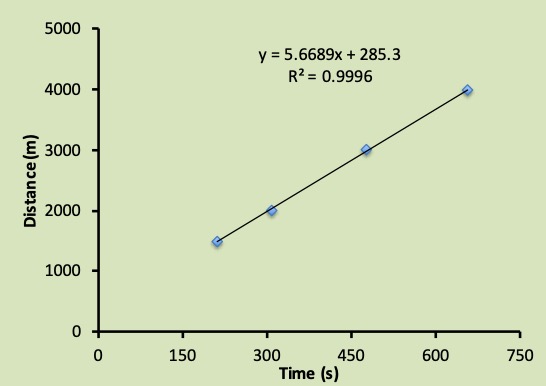
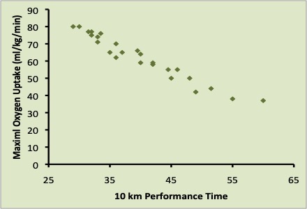
Maximal oxygen uptake (V̇O₂max) is the highest rate at which oxygen is taken up, distributed, and used by the body during whole-body exercise (Bassett and Howley 1997). The determinants of V̇O₂max and the apparent factors that limit it are addressed in Chapter 10. V̇O₂max is an important determinant of success in endurance events (Foster et al. 1978; Karlsson and Saltin 1971). Male elite endurance athletes will have a V̇O₂max of more than 75 ml∙kg^-1∙min^-1. The very highest values recorded for males are just over 90 ml∙kg^-1∙min^-1. Females typically have slightly lower values with elite female athletes scoring above 60 ml∙kg^-1∙min^-1 and extreme values just over 80 ml∙kg^-1∙min^-1. Although V̇O₂max represents the upper limit of aerobic metabolism, exercise at this intensity already has substantial non-aerobic contribution. It is thought that there is a finite amount of non-aerobic energy available, so once this energy is expended, this intensity of exercise can no longer be sustained. The limit of endurance at V̇O₂max is just 5-7 minutes (Billat et al. 2000). In Figure 16.2, this duration would correspond with the 2000 m time-trial for Jake (305 s), who has a oxygen uptake of 84 ml∙kg^-1∙min^-1.

Clearly, Jake’s success in running the 10 km distance is not because he uses his high V̇O₂max during the event. However, he can run the full 10 km time-trial using a high fraction of his V̇O₂max, so having a high V̇O₂max allows him to maintain a high rate of production by aerobic metabolism at this high fraction of his V̇O₂max.

A high V̇O₂max is dependent on a high maximal cardiac output and a large arterio-venous oxygen difference. These criteria for a high V̇O₂max can be inferred from the Fick equation, which is based on the principle that the amount of substance taken up by an organ (or organism) is equal to the amount delivered minus the amount coming out” (see equation 16.1). Since oxygen uptake (V̇O₂)  is the product of cardiac output and arterio-venous oxygen difference, Jake must have a high maximal cardiac output and be able to extract oxygen from his blood in order to achieve a high arterio-venous oxygen difference. Although some physiologists would use this equation to support the notion that cardiac output limits

Where a and v̅ represent arterial and mixed venous O₂ content and Q̇ is cardiac output.

Considering the broad range of values for oxygen uptake in the human population V̇O₂max is clearly a distinguishing feature that assists in identifying potential elite endurance athletes (see Figure 16.3). However, among a group of elite runners V̇O₂max is not a distinguishing characteristic (Saunders et al. 2004). This lack of apparent relationship is because all elite endurance athletes will have a high V̇O₂max and one of the important contributors to a significant correlation is a wide range of values in the corresponding variables. Running economy and oxygen uptake at have greater predictive capabilities (Costill et al. 1973; Coyle et al. 1992; Xu and Montgomery 1995). These two parameters of athletic performance are described next.

Economy of Running

Economy of running is a measure of the energy cost to travel a given distance or the rate of energy use while running at a given speed. It is easy to imagine that body mass would be a factor that would influence running economy. A simple analogy is to compare the energy cost of driving a small car versus a full-sized pick-up truck. The pick-up truck requires more gas to travel a given distance. Economy of automotive travel is expressed in terms of litres (of gas) per 100 km (or miles per gallon). The truck might require 12 litres per 100 km while the small car can travel for 6.5 litres per 100 km. This difference in economy would be reduced if the fuel use was expressed relative to mass, but there would still be differences. Part of the reason for the difference in fuel economy is due to size of the vehicles but other factors contribute – the size of the engine, shape of the vehicle etc. Similarly, the economy of running is affected by body size and other factors (see below). It makes sense to express economy of running in units of energy per distance travelled per kg of body mass, but this approach is not always used.

It is common to measure oxygen uptake to obtain an estimate of the energy used by an athlete. Often the calculation of oxygen uptake is as far as the estimate is taken, and economy is expressed as ml∙min^-1∙kg^-1 while running at a given speed. However, this expression of economy has 2 problems:

• Comparison between individuals requires that they run at the same speed
• The energy yield per volume of oxygen can vary as the substrate mix changes

The first of these problems can be overcome by expression of the economy as or ml∙km^-1∙kg^-1 but this does not solve the second problem. To address this second issue, it is necessary to express economy as kcal∙km^-1∙kg^-1 (Fletcher et al. 2009). Arriving at this estimate still requires measurement of oxygen uptake and carbon dioxide output to facilitate calculation of the energy yield per litre of oxygen used. Normal values for economy of running range from 0.95 to 1.25 kcal∙km^-1∙kg^-1.

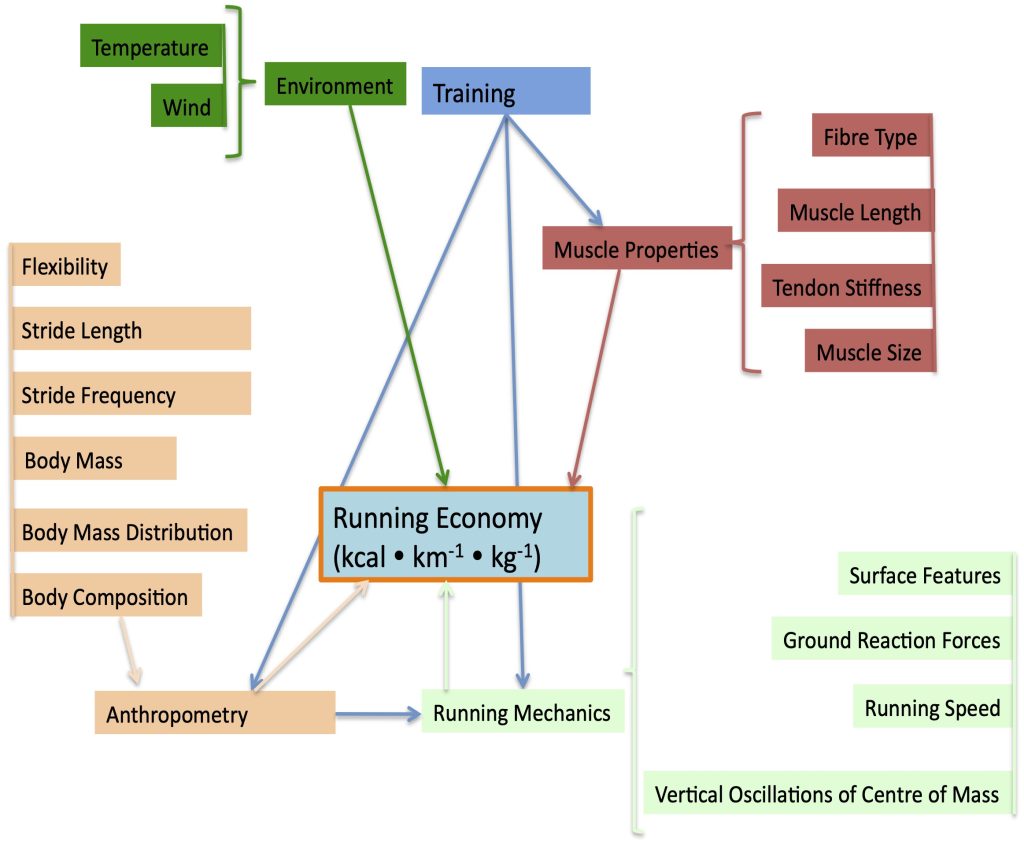
The factors that affect economy of running are not well understood, but this situation is changing (Fletcher and MacIntosh 2017). Some of the factors that affect economy of running include the following: muscle fibre-type distribution, tendon compliance, limb length, stride length, and stride rate as well as speed and load (body weight, and mass distribution). Each of these factors can increase or decrease the energy cost of muscle contractions required for running. Below, we will see how these factors influence running economy. Figure 16.4 illustrates the impact of several factors on running economy. Some of these factors are obvious and will not be discussed here. Others including muscle fibre types, muscle efficiency, and tendon compliance require some explanation.

Muscle Fibre Types

Muscle fibre types were presented in Chapter 5. In that chapter, it was indicated that muscle fibre types can be categorized on the basis of contractile, histochemical, and protein isoform properties. Adult human muscle has three categories of fibre type (type I fibres, type IIa fibres and type IIx fibres), but it is recognized that intermediate types do exist in the form of hybrid fibres. Foster et al. (1978) evaluated biopsies from 26 runners with a broad range of skill and found that % slow-twitch fibre composition was significantly related to endurance running performance. Furthermore, they present data from previous studies that confirm this relationship. Jake is a highly successful endurance runner so it would be expected that he would have a high proportion of type I muscle fibres in his legs. If we were to take a biopsy of his gastrocnemius muscle, we would likely see >75% slow-twitch muscle fibres. The remaining fibres would be hybrid Type I-Type IIa, and Type IIa. He would likely have very few if any Type IIx fibres.

It could be asked whether this high proportion of slow-twitch fibres is genetically endowed or a consequence of training. Although there is a long history of belief among exercise physiologists that muscle fibre type cannot change with training, this belief has been successfully challenged. It has been known for quite a long time that muscle activation pattern is primary determinant of myosin isoform expression and that cross-reinnervation (Buller et al. 1960; Luff 1975) or imposed electrical stimulation of the appropriate pattern (Pette and Staron 2000) will induce a change in myosin isoform expression. However, these are artificial ways of modifying muscle fibre type. The relevant question is whether voluntary activation associated with training can achieve the same fibre type transformation.

Coyle et al. (1992) reported that % slow-twitch muscle fibres was correlated with years of endurance training and Rusko (1992) has demonstrated that endurance training can cause a shift towards slow-twitch muscle fibres in elite cross-country skiers. This latter study presents rather convincing evidence for a training-induced change in fibre type expression.

Rusko (1992) evaluated muscle biopsy samples from elite cross-country skiers before and after 8 years of high training volume. He observed an increase of type I muscle fibres of 11% over the eight years, nearly 1.5% per year. Athletes who retired at the time of the initial measurement were also measured 8 years later and they were found to have decreased in type I fibre proportion. The implications of this research are clear. Fibre type can and does change with training, but the changes occur very slowly. It takes years of high-level training to achieve a noticeable change in fibre type composition. The fact that this fibre type transformation is very slow provides an answer for why most research studies lasting 8-20 weeks find no significant change in fibre type.

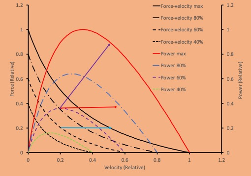
How can fibre type affect the energy cost of running? Understanding the energetics of skeletal muscle is complex. There are some generalizations that will make this understanding of energetics easier. The easiest way to consider the advantage of slow-twitch fibres is to consider isometric contractions. Slow-twitch muscle fibres contain a myosin isoform that has a relatively slow rate of use. This slow rate of ATP use relates to the fact that crossbridge of slow-twitch muscle fibres remain attached longer than crossbridges of fast-twitch muscle fibres. This longer time of attachment causes the slower rate of ATP use. The same force is maintained for a lower energy cost in slow-twitch fibres. During fast velocity shortening, this advantage is lost in that cross-bridge turnover increases in proportion to velocity of shortening. The force generated by slow-twitch fibres decreases more than the force generation of fast-twitch fibres due to the force-velocity relationship (see Chapter 5). Fast-twitch fibres become an advantage when shortening velocity is fast, but when shortening velocity is slow, then slow-twitch fibres still retain an advantage over fast-twitch fibres. This advantage becomes clearer when efficiency of contraction is considered.

Efficiency of Muscle Contraction

Mechanical efficiency is defined as the mechanical work accomplished divided by the total energy used. Efficiency can also be quantified as the power output divided by the rate of energy input. Either way, this calculation is essentially an expression of the relative conservation of energy in a useful form. When the work accomplished and the energy used are both expressed as kcal, or joules the ratio has no units. Efficiency is typically expressed as a % by multiplying this unitless ratio by 100.

Efficiency is easy to calculate for tasks like cycle ergometry where whole body exercise results in substantial work. The total energy input is estimated by measurement of V̇O₂ and the appropriate consideration of the substrate that was metabolized as discussed earlier in this chapter. However, efficiency is not easy to calculate when work or power is not easily quantified, as is the case in running. Once Jake reaches a relatively constant running speed, the work he is doing is the work to overcome air and ground resistance. This impediment to forward motion is a combination of the resistance due to motion through the air as well as the intermittent resistance associated with each foot-strike. The energy associated with this work is a small proportion of the total energy input which is calculated from the measurement of the and production. The “efficiency of running” is typically very low and is probably meaningless because “work” is not the objective, locomotion is.

It is a curiosity that running at a fast speed requires considerable energy, but output is not very high. This low power output is because lateral translation of a body requires very little work. In fact, if we add work to the task of locomotion by increasing the vertical oscillations of the centre of mass with each stride, the energy cost of running will increase, even if speed of forward movement is not changed. Jake has a nice smooth running style with very little vertical oscillation of his centre of mass. Paradoxically, one way to improve economy of locomotion is to reduce power at a given speed. This applies not only to the idea that vertical oscillation of the centre of mass needs to be minimized, but also relates to modes of locomotion like skating, swimming, and cycling where resistance to forward locomotion is substantial. Reducing the resistance to forward locomotion while maintaining speed will reduce the power output but improve economy. This concept is further described in the next paragraph.

Measurable power output increases considerably when the speed of locomotion is substantial, like in cycling. Imagine someone cycling at a given speed in an upright position versus a more streamlined position at the same speed. Air resistance is greater in the upright position, so power output (resistance velocity) will be higher in this position. By bending over to a more streamlined position, air resistance will decrease and so will power output at the same velocity. Energy cost (rate of energy use) will also decrease, but not proportionally as much as power output. Reducing power in this way should reduce the energy cost to travel a given distance because speed is the same in both cases. Efficiency would go down, because power has decreased more than the energy cost, but economy would be improved. This interesting contrast between efficiency and economy is more relevant in race events with higher speed and therefore greater air resistance like cycling or speed skating. However, economy is still more important in running than efficiency is.

Tendon Stiffness/Compliance

It was recently revealed that energy cost of running was negatively correlated with Achilles tendon stiffness, and positively correlated with patellar tendon stiffness (Karamanidis and Arampatzis 2006). Stiffness is a quantitative measure of the force needed to stretch something (like a tendon). Stiffness is expressed as N∙mm^-1. Compliance is the inverse of stiffness: mm∙N^-1. The energy cost of running will decrease as Achilles tendon stiffness increases and will increase as patellar tendon stiffness increases. This observation reveals that tendon stiffness is an important determinant of energy cost, but the relationships are complex. In some cases, stiffness is better for reducing energy cost and in other cases a more compliant tendon is desirable. The actual mechanism by which these differences can help keep the energy cost of running low is not clear, but probably relates to the increasing energy cost of a muscle contraction as velocity increases (Fletcher et al. 2013b). This concept dictates that if you keep the velocity of contraction low, you will minimize the energy cost.

How can high compliance in one tendon and high stiffness in another tendon decrease the energy cost of running? Every muscle that contracts during running will have an impact on the energy cost. Any structural property that can decrease the energy cost of a muscle contraction will contribute to an improved economy and lower energy cost per distance travelled. In general, an isometric contraction has a lower energy cost than a contraction that involves shortening, if the number of motor units and number of activations remain constant.

There are very good reasons that high tendon compliance in one muscle group (quadriceps), and low tendon compliance in another muscle group (triceps surae) will reduce energy cost of running. In both cases, these tendon properties influence the velocity of shortening, and therefore will also influence the energy cost of muscle contraction. The key is to recognize that these muscles behave differently during running.

In the case of the quadriceps muscles, the muscle-tendon unit is stretched at the beginning of the stance phase of running and shortens late in the stance phase. A compliant tendon is stretched during the early phase and shortens later, allowing the muscle fibres to remain at a relatively constant length during the whole stance phase. This mechanical response has the potential to conserve energy in two ways: 1) lower velocity of length change of the muscle will reduce energy cost, and 2) energy stored in the stretched tendon is released during the latter part of the stance phase, as force decreases, and this shortening tendon contributes to forward locomotion. This latter property represents a conservation of potential energy and is often referred to as energy transfer.

The gastrocnemius muscle does not likely have a stretch phase prior to shortening, so the discussion above does not apply to the muscles of the triceps surae. In this case, it is important to recognize that even during an isometric contraction, muscle fibre shortening will occur if the tendon is compliant. Actual muscle fibre shortening can result from altered joint configuration (plantar flexion in this case), and from shortening to compensate for elongation of a tendon. A more compliant tendon will stretch more, requiring more shortening of the muscle fibres in a given time (greater velocity of shortening). In this case, a stiff tendon can reduce the need for shortening, and therefore reduce the energy cost of the muscle contraction (see Figure 16.5).

In addition to reducing the velocity of contraction, a stiff tendon will also restrict the magnitude of shortening needed by muscle fibres, permitting the muscle to remain at a sarcomere length close to the optimum. This function of the tendon permits the force generating capabilities of the muscle to remain high, according to the force-length relationship of muscle.

Economy of locomotion, the energy cost to travel a given distance, is an important determinant of success in endurance running. When a runner can go a given distance using less energy, they maintain a given speed with a lower rate of energy use. Among other factors, economy is affected by muscle fibre type, tendon compliance, and efficiency of muscle contraction. Jake’s regular run training will have brought about favourable changes in each of these factors, as well as other factors like stride length and frequency. All of these adaptations will contribute to his outstanding performance of the 10 km run.

Fractional Use of Maximal Oxygen Uptake

The term “fractional use of V̇O₂max” is often given as a determinant of success in endurance events. If the closest competitor to Jake could maintain a higher % of hisV̇O₂max at his (say, 88%), then he should be able to perform better than Jake. However, this statement would only be true if all other factors were equal between these two competitors. If his V̇O₂max was lower than that of Jake (perhaps 75 ml∙kg^-1∙min^-1), it would be fair to say that Jake would still be the better runner. An even more revealing way to use threshold would be to express it as a speed. The term critical speed is a term that takes this notion into consideration. In fact, the critical speed incorporates the metabolic rate that can be sustained for a long time and the economy of locomotion into one term, making this the best predictor of success in a 10 km run. To fully understand the determinants of success, it is important to consider these parameters independently and yet to understand that they all work together to dictate the best performance an individual is capable of.

Anaerobic Capacity

Understanding that the term “anaerobic” means “without the use of oxygen”, it is useful to imagine that the term “anaerobic capacity” refers to the total amount of energy that can be derived without the use of oxygen. In practical terms, anaerobic energy refers to the energy that comes from net degradation of , and PCr, and from glycolysis leading to formation of or pyruvate that accumulate in the body. It is generally assumed that there is a constant (fixed) amount of energy that can be provided by these mechanisms for a given individual.

Maximal Accumulated Oxygen Deficit

In contrast with supra-threshold exercise, one of the unique features of the is that it represents a pseudo-steady-state. At or below this intensity of exercise, the physiological response is able to keep several blood and muscle constituents at a constant level. For example, blood and oxygen uptake remain constant. However, when the exercise intensity exceeds the threshold, an unsteady-state exists. The body will accumulate lactate and the oxygen uptake may continue to increase even if the speed of running does not change. Once he begins running at a speed greater than his critical speed, Jake is tapping into his limited non-aerobic energy reserves. Considering these energy reserves are limited, there is only a finite distance that he can run at a speed greater than the critical speed. This finite distance is equivalent to the intercept of the linear relationship between distance and duration shown in Figure 16.2. In this case, Jake can travel a distance of 285 m using exclusively non-aerobic energy. This anaerobic capacity is quite low in comparison with sprinters or even average active students; however, it is typical of highly trained distance runners. Knowing his economy of locomotion (see below), this distance can be used to calculate a finite amount of energy. This energy would be his anaerobic capacity. Anaerobic capacity can also be determined with the test described in this chapter’s Research Feature.

It is important to realize that the energy associated with anaerobic capacity is over and above the aerobic energy associated with critical speed (or threshold). Consider the following example to see how these energy sources work together.

Jake has an anaerobic capacity (distance) of 285 m and has run most of his time-trial at his critical speed. If he has used only half of this capacity during parts of the race, he will have half of this anaerobic capacity still available for a finishing kick (142.5 m). Although non-aerobic energy would have been required during the initial minute or two (oxygen deficit), this energy is not considered part of the anaerobic capacity determined by the critical speed test. If Jake picks up the pace by 2 m∙s-1 over the final 71 s, he could completely deplete his non-aerobic energy by the end of the time-trial and finish the time-trial in less time than if he had maintained his critical speed to the finish. The ability to increase the pace during the final stage of a race is dependent on whether or not the runner has expended their anaerobic capacity during the race. If no anaerobic energy is left, then an increase in pace is not possible.

Sprint Versus Endurance Performance

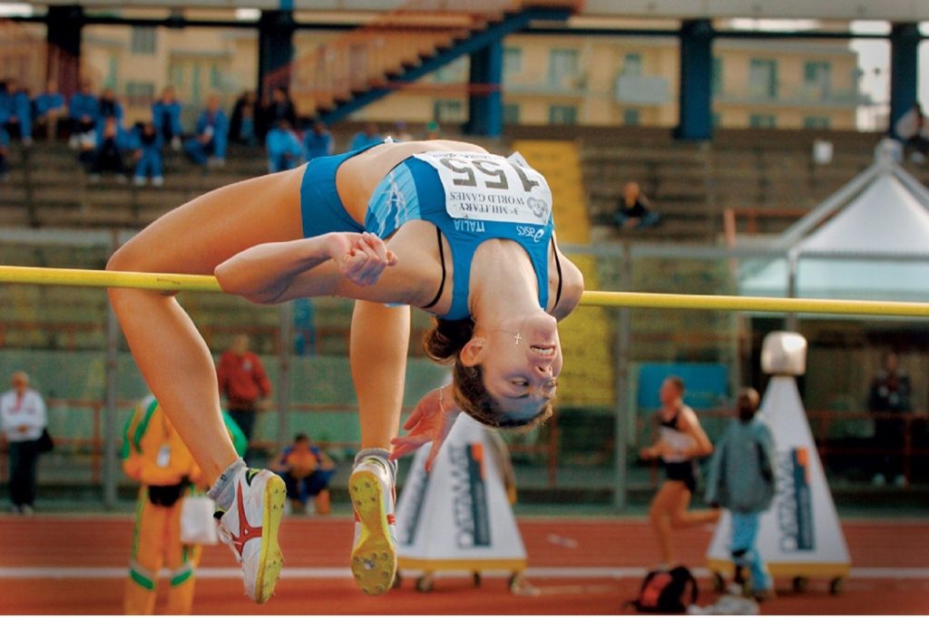
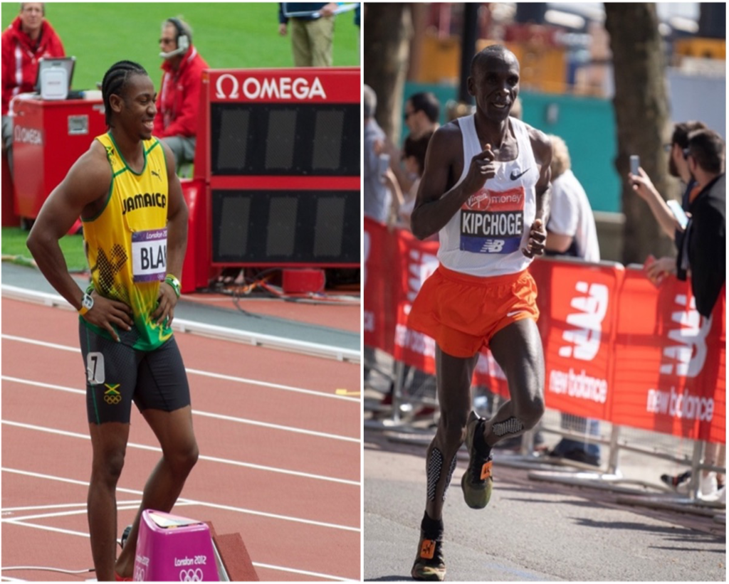
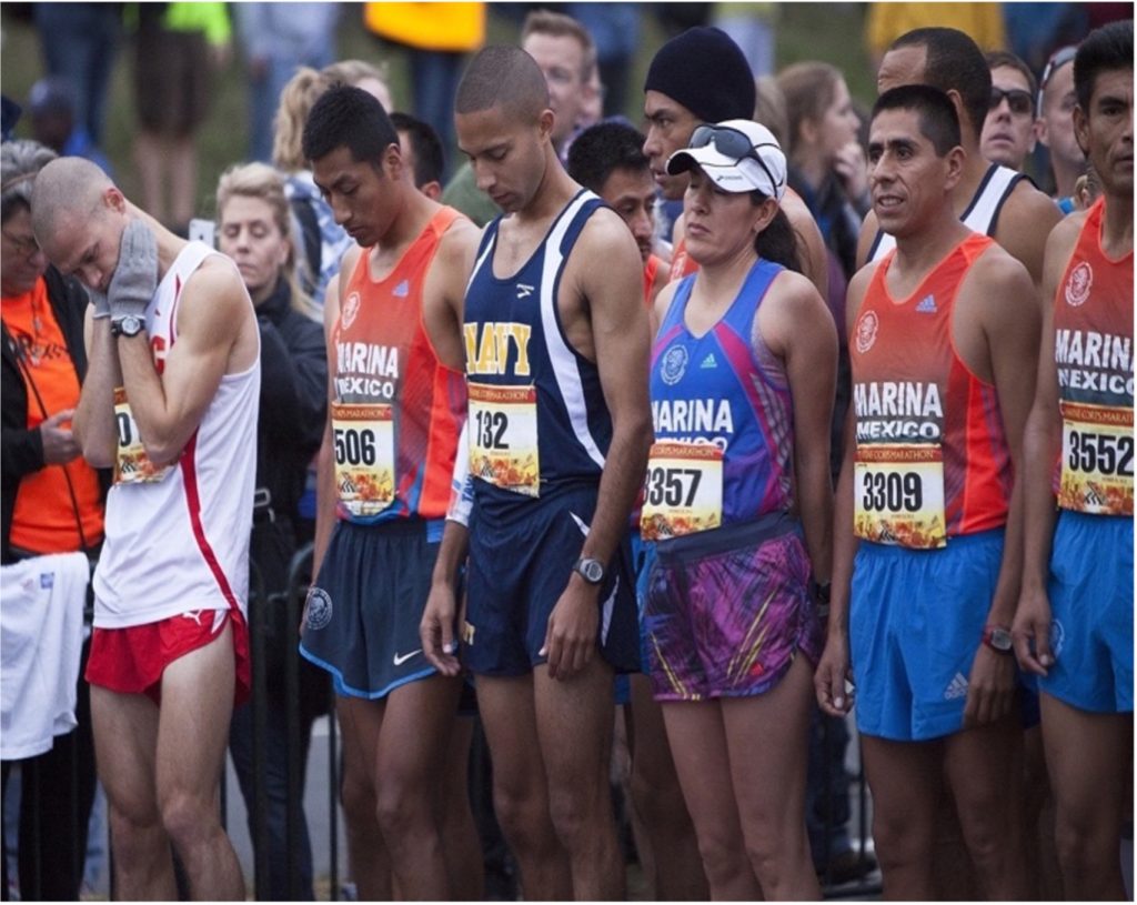
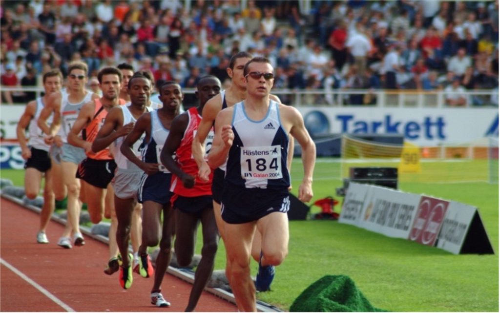
Automobiles designed for drag racing have different physical characteristics than those designed for longer duration events such as Formula 1 racing or the 24 hours of Le Mans Grand Prix. Similarly, the physical features of sprinters and endurance runners are quite different. For our purposes, a sprint event could be considered any race that is completed in less than 60 s. In sprint events, raw and maximizing the rate of energy delivery are critical. Power is defined as the rate of doing work (force∙distance∙time^-1). In endurance events which last longer than 60 s (and sometimes several hours or even days!), economy of locomotion and maintenance of a steady-state at a high sustainable rate of energy delivery are more critical. It is not surprising that the physical appearance and physiological characteristics of sprint runners (see Photo 16.3) are quite different from those of endurance runners. Sprinters require large powerful muscles while endurance runners want to minimize body mass. There are also qualitative differences. For example, sprinters have a large proportion of muscle fibres that are fast-twitch while endurance runners have a greater proportion of slow-twitch muscle fibres. A detailed description of these fibre-types was presented in Chapter 4. The implications of these fibre types will be described later in this chapter.

The greatest physiological differences between a sprinter and an endurance athlete can be summarized as the difference between an athlete who relies primarily on non-aerobic energy sources and one who relies on aerobic energy sources. The sprinter needs to provide at a very high rate for a short duration of time. This can be achieved most effectively by non-aerobic metabolism: glycogenolysis, glycolysis, and PCr hydrolysis, which provide energy very rapidly. All of these processes happen within the active muscles themselves. In contrast, the endurance athlete must rely primarily on aerobic metabolism. The maximum rate that energy can be made available with aerobic metabolism is just a fraction of the rate that can be attained with non-aerobic metabolism, but aerobic metabolism can be sustained for a much longer period of time. This is why the endurance athlete has a big heart, a highly developed vascular system, and a greater relative volume of in their muscles. Another physical difference between the two athlete-types is that endurance runners have a larger surface area-to-mass ratio than sprinters. This provides an advantage in heat dissipation, as described later in this chapter. Heat dissipation is not as important for sprinters because they do not sustain their intense exercise for as long as endurance runners do and are therefore at a much lower risk of overheating.

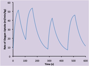
Oxygen Uptake Pattern in Ice Hockey

We have seen that the pattern of during a race or time-trial event has three phases: transition, steady level, and recovery. The pattern of oxygen uptake would be very different from this for an intermittent activity like that expected during an ice hockey game (see Figure 16.6). In hockey, the players take turns participating in the game, and these bouts of physical exertion are separated by periods of rest while team-mates get their turn. While a player is on the ice, intensity of exercise is quite high, often in excess of the intensity associated with maximal oxygen uptake. When the metabolic cost of exercise exceeds the maximal oxygen uptake, it is referred to as supramaximal. This supramaximal exertion in hockey continues for 30-60 s and is commonly followed by a rest of 1-4 min. Remembering that oxygen uptake takes time to rise following an increase in exercise intensity (the transition phase), V̇O₂ is unlikely to rise all the way to its maximum during the 30-60 s on the ice. The time to reach maximum is typically in excess of 60 s, and the player would normally be back on the bench before their V̇O₂ reaches the maximal level. Alternatively, when a player does stay on the ice more than 45 s, the supramaximal intensity is not typically maintained, and V̇O₂max is not required. In this circumstance, it would be expected that V̇O₂ would oscillate at a higher level, as in the third increase in V̇O₂ shown in Figure 16.6. While sitting on the bench, the player’s would fall exponentially towards the resting level, but would not reach resting oxygen uptake in the 2-4 min available before the next bout of exertion. This declining V̇O₂ is called recovery V̇O₂. The resulting oscillations in V̇O₂ for the hockey player would look something like that shown in Figure 16.6. Note that the concepts of aerobic inertia and EPOC (excess postexercise oxygen consumption) apply to the hockey player, just as they do for Jake (see below). However, there is no “steady level” phase of V̇O₂, and no discernible slow component of oxygen uptake. These are absent because the hockey player does not stay on the ice long enough to develop these.

—

Gender Feature:  Male Versus Female Endurance Performance

When we are considering the determinants of success in athletic events, it is also relevant to consider other factors that determine male vs female differences in exceptional performance.

During the 1980’s, experts predicted that women would surpass men in performance of long-distance events like the marathon, a running race that covers 42.2 km. This prediction was based on extrapolations of the history of marathon performance records. Figure 16.7 illustrates the history of world records for males and females for the marathon. It is obvious that prior to the 80’s, marathon records of males and females were converging very quickly. This convergence was due to the rapid improvement of records for females, whereas the male world records improved at a much slower rate. It is easy to see how someone looking at the records in the 80’s might surmise that females will one day overcome males in this sport. However, this extrapolation of information from the graph (Figure 16.7) can obviously be misleading.

Since the 1980’s, the rate of improvement of records for females has changed to a rate that is not substantially different from the rate of change of records for males. Although their performances are much more similar now than they were just 30 years ago, it seems much less likely that females will eventually beat the males. While it is speculative to indicate why these rates of change have evolved in the way they have, it is worth considering what might have allowed females to improve much more quickly than males during the early 80’s. The main reason is most likely sociological. As more females participate in sports events, there will be more great performances. You will notice that the world records for females in the marathon started in the 1950’s, but men were doing the marathon much longer than that. Women were not allowed to compete in this distance until well after the men had achieved respectable performances. It is important to understand background relationships like the time course of world records before useful extrapolations of this data can be done.

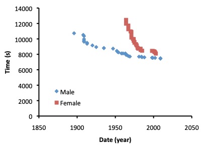
In contrast with the comparison of male and female endurance runners, comparisons of top performances (not simply records) for male and female sprinters have revealed that the difference between the sexes is actually increasing. The increasing difference in performance is actually due to slowing of top performances of women in the past few years. This anomaly has been proposed to be a function of the decreased use of anabolic androgenic steroids among the world’s top female sprinters. Anabolic steroids are in a class of drugs that promo

ynthesis, leading to increased muscle mass. These drugs are illegal to use without a medical prescription and are banned by the World Antidoping Agency, due partly to the unfair advantage obtained but also because of side effects with serious health implications.

This interesting speculation on changing drug use is described in detail at sportsci.org. Additionally, an interesting analysis of Masters records for a variety of distances is given at eliteracingsystems.com.

There are several key physiological differences between males and females that will always contribute to the differences that are evident in Figure 16.7. The principal factors that make males faster than females relate to sex-specific differences in muscle mass and mass. Females typically have more body and less muscle than males, though this difference is much smaller in elite distance runners than in the general population. In the case of a marathon race, having less fat is an advantage because fat does not contribute to the success in the event, rather, extra body fat increases the absolute energy cost of locomotion. Although females can add muscle mass with weight training, the use of anabolic steroids has been a tempting option for some. The recent move to eliminate this practice has resulted in slowing of sprint performances in world class female sprinters over the past several decades.

It is interesting to note that there appear to be no significant differences in running economy between males and females (Fletcher et al. 2013a). However, some investigators still claim that females have better economy than males (Mendonca et al. 2020), this observation relates to the inappropriate use of a slight grade on the treadmill in an attempt to simulate over-ground running, which has a slightly higher energy cost than running on a treadmill. This modification penalizes those with higher body mass, so males tend to have a higher energy cost of running than females when this is done.

Aerobic capacity (maximal oxygen uptake), one of the key physiological determinants of success in endurance events, is typically expressed per kg of body mass. Muscle tissue contributes to the capability to use oxygen, but fat does not. For a given mass of muscle, a body with more fat will have a lower relative V̇O₂max. This is evident in Table 16.1 when you compare Jake with Rachel. Note that Rachel’s V̇O₂max is less than Jake’s, but still higher than Andrew’s. As well, females typically have a smaller lung volume than their male counterparts, which results in a lower maximal absolute V̇_E.

Now that we have considered some of the sex-specific differences and the differences between sprinters and endurance athletes, it is time to proceed with a discussion of the physiological responses during an incremental exercise test. This information will help put the determinants of success in perspective. The description of the physiological responses that is given below is presented with consideration for Jake’s physical and physiological characteristics that are presented in Table 16.1.

—

Physiological Response During a 10 km Time-Trial

This part of the chapter will focus on the physiological responses that would be expected for Jake if he were to begin the time-trial by accelerating to the speed that he hopes to maintain for the duration of the event and holds that pace until the finish. This is the strategy, called “even-splitting”, that will permit Jake to complete the distance in the shortest possible time. It is important to realize that there are three distinct physiological phases to the race, deemed the transition, steady pace, and recovery phases. The physiological responses in the body are quite different during these three phases. In reality, a fourth phase might be relevant -the “end-spurt” or “kick”, where competitors finish a race or time-trial with an increase in speed above the average speed maintained through-out the race.

Oxygen Uptake

Oxygen is necessary for aerobic metabolism. Oxygen is taken into the body via and pulmonary gas exchange (see Chapter 7) and is delivered via red blood cell circulation to the tissues throughout the body. Oxygen is needed in the for phosphorylation. Oxidative phosphorylation is a process that provides adenosine triphosphate (ATP) to meet the increased demand for energy by the active muscles. The rate of phosphorylation relies on the availability of oxygen. At rest, the body needs about 3.5-4.0 ml∙kg^-1∙min^-1 of to satisfy all energy requirements. When metabolic rate increases due to muscle contractions during exercise, there must be increased delivery of oxygen to the muscle cells. The measurement of V̇O₂, and the various phases associated with the kinetics of oxygen uptake were presented in Chapter 6. These are relevant to the current chapter.

At the beginning of his time-trial, Jake is still in the recovery phase from his warm-up. His oxygen uptake at the start line will possibly have returned to his usual resting state. One of the key benefits of a warm-up is that the kinetics of oxygen uptake are accelerated by prior exercise (Burnley et al. 2002). This faster rise in rate of oxygen uptake will reduce the amount of energy that must come from non-aerobic metabolism during the transition phase following exercise onset. We will see from the determinants of performance described below that any time we can provide energy via oxidative metabolism rather than from non-aerobic metabolism, there is a benefit. This is particularly true during the transition to the steady pace because this reduces the oxygen deficit – the cumulative difference between total energy required and the energy provided by aerobic metabolism. This energy, referred to as the oxygen deficit, is provided by non-aerobic metabolism, and it is thought that there is a limited supply of non-aerobic energy. Any delay in using this limited supply can permit better performance later in the time-trial.

Supply and Demand

It is important to realize that in the skeletal muscles, there are two important factors that dictate the relative contributions of aerobic and non-aerobic metabolism: energy demand vs energy supply. Keep in mind that both metabolic systems are attempting to replenish as fast as it is used. We know that [ATP] does not decrease substantially during endurance exercise, so this balance is maintained by replenishment (via both aerobic and non-aerobic metabolism) matching ATP hydrolysis by the three key ATPase enzymes: actin-myosin-ATPase, Ca²⁺ATPase and Na⁺–K⁺ATPase. Skeletal muscle contraction dictates the demand, or rate, of ATP usage, and oxygen delivery and mitochondrial capacity determine the supply of aerobic energy. When [ATP] remains constant, non-aerobic pathways provide the additional ATP.

Transition Phase

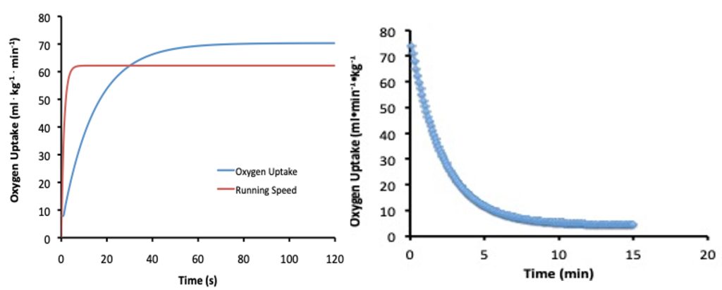
At the beginning of his time-trial, Jake will accelerate to the speed that he wants to maintain for the majority of the distance. This acceleration will take only a few seconds which means his actual energy requirement will increase rapidly relative to the speed he is running, with extra energy needed for acceleration. In contrast, will have slower kinetics. The rate of V̇O₂ will increase from just slightly greater than a normal resting level to a level that would nearly support the metabolic demand for energy after about 1-2 min. This increase in oxygen uptake is illustrated in Figure 16.8. The fact that oxygen uptake require s a minute or more to reach the steady-state is called aerobic inertia, but the mechanism of this slow increase is not clear.

Following exercise onset, it can take several minutes for oxygen uptake to reach a steady-state in a less well-trained individual. One view on the reason for this aerobic inertia is that the rise in oxygen uptake occurs slowly because non-aerobic energy pathways are activated more quickly, and these processes replenish nearly as fast as it is required in the muscles (Lanza et al. 2005). Alternatively, the more traditional view is that rapid acceleration by Jake to the speed that he will maintain during the time-trial will use ATP faster than aerobic metabolism can initially replenish it. The difference between these explanations is subtle. In one case, the slow rise in V̇O₂ is due to the slowed decrease in [ATP], due to contributions from non-aerobic pathways. In the other case, the activation of non-aerobic metabolism is thought to compensate for a slow delivery of oxygen. Non-aerobic metabolism will make up the difference in either case, preventing much decrease in ATP concentration. Non-aerobic metabolism includes hydrolysis of PCr, and glycolysis leading to the formation of lactate. There is also some non-aerobic energy provided by a small net breakdown of ATP. However, the concentration of ATP within a cell is never permitted to decrease very much, as the cell’s viability depends to a great extent on the availability of ATP. The non-aerobic energy makes up the oxygen deficit.

As increases, the rate at which ATP is provided from the non-aerobic pathways is slowed, and concentration in the active muscles is maintained at a concentration just slightly lower than the resting value. Phosphocreatine (PCr) concentration decreases substantially during the time that oxygen uptake is increasing. This decrease is evidence that PCr hydrolysis contributes to the energy needed for the exercise. If the pace was slow enough to permit oxidative metabolism to provide all of the energy at steady-state, the oxygen deficit would only accumulate during the time that oxygen uptake was rising. However, since Jake will be running at a pace that is above his , the oxygen deficit will continue to accumulate throughout the time-trial, and by the finish should have reached what would be his oxygen deficit (see Chapter 13).

Steady Level Oxygen Uptake and the Slow Component

It should be kept in mind that the changes in and phosphocreatine concentration will only be in the motor units that are active. Running at his race pace will not initially require Jake to activate all of his motor units in the muscles that can be used for running. Also, of the active motor units, only a few will be maximally or near-maximally activated. For most of the time-trial, Jake will maintain a nearly constant oxygen uptake while running at his race pace which is just slightly faster than his critical speed (see intensity-duration relationship, illustrated in Figure 16.2). However, in spite of the constant pace, there will be a continued slow increase in oxygen uptake for the first 10-15 min. This slow increase in V̇O₂ is due to the slow component of oxygen uptake. The slow component of oxygen uptake is the reason that the initial value for V̇O₂ in the graph on the right side of Figure 16.8 begins at a higher value than indicated by the end of the graph on the left. The concept of the slow component of slow component of oxygen uptake was covered in Chapter 13 The actual mechanism responsible for this increasing V̇O₂ is not fully understood. It could represent a decreasing non-aerobic contribution that is compensated for by an increasing V̇O₂ , 2017b) Most exercise physiologists believe the slow component is associated with fatigue, and the need to recruit less efficient (or in this case, less economical) motor units, and/or support an increasing minute ventilation, which is typical of continued exercise at an intensity above the . However, this seems unlikely.

During his time-trial, Jake is running at a pace just above the threshold. He will be hyperventilating and blowing off more CO₂ than his cells are producing. However, based on studies using radioactive-labeled substrates and understanding his level of training, it is reasonable to assume that he will provide no more than 30 % of his total required energy with oxidation of fats. Fats and/or COH can be labelled with radioactive carbon or hydrogen to allow monitoring of the amount of these substrates oxidized during exercise. This technique is not affected by the that alters pulmonary CO₂ output, so it offers precision even above the threshold.

When the mix of substrates metabolized and the <a class=”rId256″ title=””a measure of the rate of use of oxygen in the body, or part of the body by detection of the difference between O₂ inhaled and O₂ exhaled”” href=”https://kinesiology.ucalgary.ca/macintosh/glossary/max-ph#v-%CC%87o2–“>V̇O₂ are known, then the total amount of COH metabolized can be estimated. This is important because the total amount of COH available in the body can be a limiting factor in performance of endurance events (Karlsson and Saltin 1971). The total amount of COHs that Jake needs for this time-trial (nearly 220 g; see Highlight Feature 16.1) would represent approximately 70-80% of the total COH stores (muscle and liver glycogen as well as free glucose) available to Jake prior to the time-trial. There would be no need for him to undergo procedures for “carbohydrate loading” or to consume COH during the event. Carbohydrate loading is a training and dietary procedure that is intended to enhance the total COH content of the body by increasing muscle glycogen storage (James et al. 2001; Nakatani et al. 1997).

Some of the substrates metabolized in Jake’s muscle will come from stores within the active muscle cells, but some will be taken up from the blood flowing through the capillaries adjacent to these cells.

In order for Jake to get the substrate needed for oxidative metabolism into the blood where they can be delivered to and taken up by his active muscles, it is necessary to remove the and COH from storage sites in his body. Although Jake is very lean (see Table 16.1), fat is stored in Jake’s adipose tissue in the form of triglycerides. Carbohydrate is stored in muscle and liver in the form of glycogen. Substrate mobilization, the process of getting these substrates out of storage and into the blood, is triggered by hormones. Catecholamine, growth hormone, glucagon, and cortisol are critical hormones that perform this function. The concentration of these hormones in the blood can be increased in response to a decline in blood glucose. During exercise, the concentration of these hormones also increases in anticipation of Jake’s need for more fuel for the time-trial. This is an example of a feed-forward control system.

The hormonal response during Jake’s time-trial will permit him to use a mix of COH and as fuel for his run, without depleting his muscle stores of glycogen. He will experience increases in epinephrine, norepinephrine, glucagon, growth hormone, and  cortisol in his blood. The response of these various hormones will be moderate, since the exercise intensity will be just slightly higher than his intensity at anaerobic threshold. The increases will be less than in a less trained individual running at the same speed. The consequences of the increase in catecholamine, cortisol, glucagon, and somatotropin concentrations will be an elevated rate of output of glucose from the liver such that Jake will not deplete his glycogen stores in the primary muscles used for running. However, glycogenolysis will still be going on in those muscles. Glycogenolysis will also be occurring in his inactive muscles, stimulated by the increased sympathetic nervous system. Since oxidative metabolism in these muscles is relatively low, will be produced and will move into the blood, contributing to the increase in blood lactate concentration.

In this example, we are assuming that Jake will run almost the entire time-trial at a constant speed. An alternative strategy would be for him to run at a slightly slower speed for much of the time-trial and pick up the pace near the finish. If he did this, he would experience a rise in oxygen uptake near the end of the time-trial. HisV̇O₂ can rise no higher than his maximal oxygen uptake, so his non-aerobic energy pathways must help replenish the ATP that he uses, not only during the time that oxygen uptake is rising, but also after that if his demand exceeds the rate of his aerobic ATP replenishment.

The shape of the graphs in Figure 16.8 would be very similar for a female distance runner (like Rachel). However, the speed of running would be slower and the magnitude of V̇O₂ would be correspondingly lower. There are several reasons contributing to the slower running for Rachel, some of which are not fully understood. One factor that contributes to the slower running is that Rachel has a higher energy cost of running than Jake has, shown in Table 16.1. Rachel requires 1.01 kcal·kg^-1·km^-1 whereas Jake can run while using just 0.96 kcal·kg^-1·km^-1. This means that even if they could maintain the same relative V̇O₂ for the duration of a race, Jake would be going faster than Rachel. Rachel will also most likely have a higher body content than Jake. This means that her muscle mass represents a slightly smaller proportion of her body than Jake’s muscle mass of his body. Since muscle mass is a primary determinant of absolute V̇O₂max, this smaller relative muscle mass contributes to a lower V̇O₂max.

Recovery Oxygen Uptake

The graph on the right in Figure 16.8 shows that Jake’s V̇O₂ begins to decrease once he completes the time-trial, but the decrease does not go immediately to his resting level. If Jake were to completely stop at the finish line, and lie down, his oxygen uptake would still not immediately return to a resting level. Even simply walking around, Jake’s oxygen uptake would take considerable time to return to a steady rate that would resemble the V̇O₂ at rest. This is evident when watching racers gasp for air after finishing a race. Jake’s V̇O₂ would decrease exponentially after exercise and would take 20-60 minutes to reach a constant level (Short and Sedlock 1997). Some research indicates that it would take even longer than this duration. The total oxygen uptake used by Jake’s body once he completes the time-trial is called the recovery (also known as “excess postexercise oxygen consumption” or EPOC). V̇O₂ does not return immediately to the resting level, because energy is needed during the recovery period that is greater than that normally needed at rest, and oxygen stores that were used during the exercise need to be replaced.

Several factors contribute to Jake’s recovery including: returning oxygen stores (haemoglobin and myoglobin) to a resting state, resynthesis of ATP , PCr, and some glycogen, and restoration of ion gradients across cell membranes. The haemoglobin that needs replacement is primarily that which is in the venous circulation. Arterial blood will have the normal amount of O₂ for the duration of the time-trial. At rest, Jake will have a venous oxygen content of about 15 ml of oxygen per 100 ml of blood. At the end of the time-trial, much of his venous blood will have an oxygen content of about 5 ml of oxygen per 100 ml of blood. Considering the venous circulation contains about 60% of the total blood volume and Jake’s blood volume will be slightly greater than the normal 8% of body mass, perhaps 9%. It can be estimated that Jake has a venous blood mass of: 0.6⋅0.09⋅61 kg or 3.29 kg. Here, 0.6 represents 60% of total blood volume and 0.09 represents 9% of body mass. Normally, blood is expressed as a volume and it can be assumed that blood has a density of 1.0, so 3.29 kg would be equal to 3.29 litres. The difference in oxygen content that needs to be replenished is 10 ml of O₂ per 100 ml of blood, or 100 ml of O₂ per litre. The total amount of oxygen uptake needed to replenish oxygen stores in the blood is 3.29 litres of venous blood 100 ml of O₂ per litre of blood or 329 ml of O₂.

A similar calculation could be made for the O₂ needed to replenish depletion of O₂ bound to myoglobin. Myoglobin is an oxygen-binding protein in muscle which is similar in many ways to haemoglobin. Myoglobin is also the molecule that gives meat a red colour. A few assumptions are necessary for this calculation. To estimate how much oxygen is needed to restore the resting state of O₂ bound to myoglobin, we need to know how much muscle is involved in the task, what the concentration of myoglobin is in the active muscles, and how much oxygen was associated with this myoglobin. Human muscles have about 2 mg of myoglobin per g of muscle. This value would be a little higher in Jake because there is more myoglobin in muscle fibres with a higher oxidative capacity, and Jake, as an elite endurance athlete, has a higher proportion of type I and type IIa fibres than most people. The total amount of oxygen stored in Jake’s active muscle would be about 0.17 mmoles per kg of muscle. If we assume that Jake has 20 kg of active muscle during his run, then this amount of muscle would have about 3.4 mmoles of oxygen. This is equivalent to 75 ml of oxygen. Since myoglobin typically loses about 70% of its oxygen during vigorous exercise, Jake would probably require just 50 ml of oxygen to replenish his myoglobin oxygen stores.

It takes several minutes for to return close to the resting level, so the metabolic needs of the ventilatory muscles would also contribute to EPOC. Similar to ventilation, cardiac output slows gradually. Extra energy is needed to maintain this extra work of the heart. The elevation in body temperature may also contribute to the elevation of during the recovery period. One of the factors that could contribute to a prolonged elevation of post exercise oxygen uptake is the need for energy to restore tissue structures that might have been damaged during the exercise. This restorative energy requirement could include muscle as well as other tissues. The repair process takes hours to days to complete but raises metabolic rate such a minor degree that it may be difficult to detect. Resynthesis of glycogen to the pre-exercise level requires dietary consumption of COH and may take 24-48 hours to fully compensate for the glycogen used during the time-trial.

Pacing Strategy

For the example shown in Figure 16-8, Jake maintains a constant speed for the duration of the time-trial. This strategy is not a typical pacing strategy. Often, 10 km races are run with variable pace such that the metabolic rate is not constant but rises and falls with the pace. The leader of the race may change several times. For any runner to be able to do their best, it is important that they not allow the pace to fall below the critical speed, which is considered to be the speed that is supported by aerobic energy. This inappropriate strategy (slower than critical speed) would represent a loss of energy that would otherwise contribute to completing the race. The major difference between aerobic and non-aerobic energy is that the former represents a potential maximal rate, and the latter represents a fixed amount of energy. Brief excursions to a higher intensity that uses more non-aerobic energy results in less of this energy being available for later. However, any running at an intensity that is less than critical speed results in a lost opportunity to use energy that cannot be recovered (Fukuba and Whipp 1999).

Another important point of strategy is to realize that the energy cost to run 10 km relies on running just 10 km, which requires running exclusively on the inside lane of the track. Any running outside the inner lane will result in running a longer distance. Considering the energy cost is expressed “per km”, any increased distance in a real-life scenario will represent a requirement for more energy.

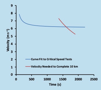
The minimum time for Jake to run 10 km can be estimated from his critical speed test. This estimation is illustrated in Figure 16.9. Here, the blue line represents his hyperbolic fit to the results of his critical speed trials (same as in Figure 16.2). The brown line depicts the time needed to cover 10 km at a given speed. The intersection represents the fastest speed that Jake can maintain long enough to complete 10 km. This speed is the pace he should use for his time-trial. Kindly note that any measurement of a threshold or critical speed will have some error. This means that the intersection here is simply an estimate and is not expected to be precise.

—

—

Cardiovascular Response

In order to deliver the oxygen that is required in Jake’s exercising muscles and to remove the CO₂ that is produced, it is necessary that his cardiac output increase well above the resting level. This greater cardiac output is achieved by increases in heart rate and stroke volume. The time course of increase in cardiac output parallels the increase in oxygen uptake that is shown in Figure 16-8. However, the magnitude of increase in Jake’s cardiac output is considerably smaller than his increase in oxygen uptake. While oxygen uptake increases about 20-fold from the true resting level, cardiac output increases only 7-fold. This increase in cardiac output will allow the greater increase in because the arterio-venous oxygen difference also increases (approximately 3-fold). In addition to increasing the cardiac output, there is a redistribution of blood flow that allows most of the extra cardiac output to go to the exercising muscles. These concepts were presented in Chapter 8.

Heart Rate

At the start line of his time-trial, Jake will very likely have a heart rate much higher than his normal resting value of 45 beats∙min^–1; perhaps about 90 beats∙min^-1. This elevated heart rate can be attributed to a combination of an anticipatory response and incomplete recovery from his warm-up. The sympathetic nervous system has already kicked in, causing the heart rate to be elevated. Once the time-trial begins, his heart rate will increase further to reach a rate of 170 beats∙min-1. His heart rate will gradually increase to nearly 180 beats∙min^-1 at the end of the time-trial in spite of the constant pace he will maintain. This gradual increase is called the cardiac drift (see Chapter 8).

It should be noted that Table 16.1 indicates that Jake will have a lower maximal heart rate than the reference male student. This lower heart rate is not simply because Jake is older. It is not unusual for a highly trained athlete to have a relatively low maximal heart rate. The reason for this lower maximal heart rate is not known. In spite of the lower maximal heart rate, Jake can achieve a higher maximal cardiac output than Andrew because he has a larger heart and therefore can eject a larger stroke volume.

Stroke Volume

At rest, Jake has a cardiac output of 4.2 L∙min^-1, and a heart rate, (HR) of 45 beats∙min^-1. Therefore, his stroke volume (SV) would be 93.3 ml∙beat^-1 (see equation 16.3). Early in the time-trial, his stroke volume will have risen to 140 ml∙beat^-1. Stroke volume would remain fairly constant at this level for the remaining duration of the time-trial. During this time, asV̇O₂ rises to nearly a maximal level, stroke volume may stay the same or increase only slightly.

Cardiac Output (Q̇) = SV⋅HR = 4.2 L⋅min^-1 = 0.0933 litres⋅beat^-1 45 beats⋅min^-1         Equation 16-3

The increase in stroke volume is accomplished primarily by an increase in the ejection fraction, which is compensated for by an increased rate of filling. The ejection fraction is the proportion of the end-diastolic volume (EDV) that is ejected, or stroke volume (SV) divided by EDV. For example, if at rest his end-diastolic volume is 148 ml he would have an ejection fraction of:

Ejection Fraction = SV ⋅EDV^-1 = 93.3⋅148^-1 = 0.683.                 Equation 16-4

During the time-trial, Jake’s ejection fraction would increase to nearly 1. Ejection fraction is illustrated in Figure 16-10.

While running at a speed of 6.22 m⋅s^-1, Jake will be generating a lot of heat which must be dissipated in order to avoid a dangerous situation like heat stroke. This heat comes from the chemical reactions that occur in his muscles to provide the energy for crossbridge formation, force generation, and ion pumping. Some of the heat comes from the reactions associated with glycolysis and oxidative metabolism, and some comes at the time each is hydrolyzed. The total heat generated can be estimated with a few basic assumptions. This estimation of heat generation during exercise is shown in Highlight Feature 16-2. This calculation shows that if there was no heat loss from the body, Jake’s body temperature could increase to above 46C! Jake could not survive with a body temperature this high, so it is imperative that he has a way to get rid of this extra heat.

—

Environmental conditions will dictate the ability to lose the heat that is generated within the body. These mechanisms of heat dissipation are described in Chapter 9 and include: radiation, conduction, convection, and evaporation. Factors that will affect the magnitude of involvement of these mechanisms include the following: air temperature, relative humidity, sources, and sinks for radiative heat loss or gain, sweat rate, body surface area, and body mass. Any heat generated that is not lost from the body will cause an increase in body temperature. This increase in body temperature would amount to 1-2C during Jake’s 10 km time-trial but could be as high as 4C during a marathon.

The amount of sweat evaporation that Jake needs to lose the extra heat he is producing can be estimated. The heat of evaporation of water is 540 kcal⋅kg^-1. Jake would have to evaporate just a little over 1 litre of sweat to lose this heat. If we assumed that he could dissipate half of the heat by conduction and convection, then only half of the heat would have to be lost by evaporation. However, some of the sweat will drop from his body or remain in his clothes at the end of the time-trial, and this sweat will contribute to fluid loss but not heat loss. He may still need to lose a litre of sweat to lose the excess heat generated in his muscles. This rate of sweat loss is within Jake’s capability.

In shorter duration events, heat dissipation is less of a problem even though heat is produced at a higher rate. For a 100 m sprint, heat may be generated at a rate that is 3-4 times greater than during the 10 km run, but this high rate of heat generation is sustained for just 10 s. The total heat generated would be sufficient to increase body temperature of a larger sprinter (80 kg) by less than 1 degree. During this sprint, muscle temperature would increase more than 1 degree because there would not be time during the time-trial for blood flow to redistribute this extra heat. The heat dissipating mechanisms are illustrated in Figure 16-11.

Blood flow is an important component of the temperature regulation process. The increased muscle blood flow that Jake would have during the time-trial is important not only for providing O₂ and removing CO₂, but also for removing this excess heat that is generated in the active muscles. The blood in the veins leaving his leg muscles will have been warmed by the passage through the heated muscles. Heat losing mechanisms rely on getting some of the warmed blood to the skin. The skin will be warmed by this blood flow and cooled primarily by convection and evaporation. A large body surface area to mass ratio will facilitate this heat dissipation.

Sweating to facilitate heat loss from the body would result in relative dehydration. If Jake was sweating at a rate of 2 litres per hour, he would lose 1.5% of his body mass during the time-trial. This fluid loss could compromise his performance and his ability to regulate temperature, so it would be important for Jake to take advantage of water stations during the time-trial.

In this section of the Chapter, we have been reminded that one of the byproducts of exercise is the generation of heat. During the 10 km time-trial, Jake will generate nearly 580 kcal of heat energy. Heat is produced in the muscles in conjunction with metabolism. The excess heat must be transported from the muscles to the skin by blood flow, and dissipated to the environment by convection, conduction, evaporation, and radiation. Of these mechanisms, evaporation is the most important for keeping Jake at a safe temperature.

Ventilatory Response

We breathe to keep the partial pressure of carbon dioxide fairly constant within the alveolar spaces of the lungs. These partial pressures allow exchange of O₂ and CO₂ between the air and the blood. As increases and cardiac output increases, there will be a need to increase to maintain these partial pressures of O₂ and CO₂.

Jake would have a resting  ventilation of about 5-6 litres. Integration of heat dissipating mechanisms.  This ventilation would involve a tidal volume of about 500 ml and a breathing frequency of 10-12 breaths·min^-1. The ventilatory response in exercise and its regulation was presented in Chapter 7. Prior to the time-trial, his ventilation would still be elevated due to his warm-up, but not by much. Jake would experience an increase in ventilation, immediately on initiating the time-trial, and a further increase would occur in conjunction with the increase in V̇O₂ (see Figure 16-8). By the time his oxygen uptake had reached 4.3 litres·min^-1, his ventilation would be well over 100 litres·min^-1. This ventilation would be achieved with a tidal volume of about 2.0-2.5 litres, and a breathing frequency of 50-55 breaths·min^-1. This rate of ventilation is more than adequate to provide the O₂ Jake needs. Hyperventilation, then, will result in a rate of removal of CO₂ from the body that exceeds the metabolic production of CO₂. Total body content of CO₂ will decline. The decline will assist with buffering of H⁺ (see Chapter 9).

Blood Lactate

Lactate is formed in muscles as a consequence of glycolysis. The enzyme dehydrogenase converts pyruvate to and at the same time converts NADH to NAD⁺. This oxidation of NADH actually permits glycolysis to continue because glycolysis requires NAD⁺. Any time there is formation of pyruvate, there will be formation of lactate in proportion to the concentration of pyruvate. Lactate is transported out of muscle cells by a monocarboxylate transporter, and H⁺ is co-transported with lactate. From the extracellular space, lactate can get into adjacent muscle cells or can get picked up by capillaries. An increased rate of glycolysis will result in increased production of lactate and increased appearance of lactate in the blood.

At rest prior to the time-trial, Jake will likely have a blood lactate concentration that is slightly higher than the concentration usually detected at rest. A normal resting level would be less than 1 mM, but Jake would have a value that was 2-3 mM. This level of “resting” blood lactate would not be due to inadequate oxygen delivery, but due to the increased sympathetic tone that would accompany the anticipation of his impending time-trial. It was presented in Chapter 6 that circulating epinephrine will activate glycogenolysis, and this increased glycogenolysis will lead to increased glycolysis. An increased rate of glycolysis will result in an accumulation of blood lactate.

Once the time-trial begins, the rate of glycolysis will be further increased, and non-aerobic metabolism will provide the additional energy needed while increases to the steady level. Blood lactate will continue to increase throughout the time-trial because Jake would be running at an intensity just above his threshold. The muscular production of lactate results in appearance of lactate in the blood. Some lactate will be taken up in less active tissue and oxidized. This process contributes to removal of lactate from the blood. However, the rate of appearance of lactate in the blood would just slightly exceed the rate of removal, so lactate will accumulate in the blood throughout the time-trial. Figure 16.12 illustrates the factors that contribute to or reduce the accumulation of lactate in the blood. By the end of the time-trial, Jake’s blood lactate concentration would be about 8 mM.

Disturbance to Ion Homeostasis

There are three key ions that are particularly important in the body and are affected by exercise: H⁺, Na⁺, and K⁺. Each of these is critical for homeostasis and important in the ability to continue exercising. The concentrations of these can vary substantially during Jake’s 10 km time-trial. The general scheme of ion exchange during exercise is illustrated in Figure 16-13. This diagram illustrates the concentrations gradients for the major ions, and the direction of transfer between the muscle cells and the extracellular space. Further exchange must occur between the extracellular space and the vascular system, across capillary walls. In Figure 16-13 an active muscle cell is shown along with an inactive muscle cell.

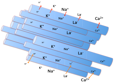
H+

During repeated contractions as would occur during high intensity running, muscle cells become acidotic. Muscle pH can decrease from a resting value of about 7.0 to 6.5 or lower, depending on the intensity and duration of exercise. During the 10 km time-trial, Jake’s leg muscles that are used for running might experience a decrease in pH to about 6.7. There is some uncertainty about the source of H⁺ that causes this acidity, but the general consensus is that it arises as a result of glycolysis and accompanies production of lactate.

The consequence of acidosis is also a controversial issue. For decades now, muscle and exercise physiologists have believed that acidosis was a primary cause of muscle fatigue. There is certainly a strong correlation between muscle acidosis and fatigue, but correlations can be misleading. A correlation can indicate a cause and effect relationship but can also occur if there is a third (or more) related variable(s). For example, consider the strong relationship between lightning and thunder. It could be that lightning causes thunder, or some other event causes both. In the case of lightning and thunder, it is another event that causes both.

Early research on the effects of acidosis on muscle revealed that Ca²⁺sensitivity is decreased by acidosis (Fabiato and Fabiato 1978). This means the force exerted by a muscle cell will be lower when the same [Ca²⁺] is achieved. This was very strong evidence that acidosis contributed to fatigue in skeletal muscle. However, more recently it has been shown that this decreased Ca²⁺ sensitivity is temperature dependent. At room temperature or lower, Ca²⁺ sensitivity is decreased by acidosis. When the muscle is warmed up to above 30C (a more physiological temperature), acidosis has little or no effect on Ca²⁺ sensitivity (Pate et al. 1995) In a genuine twist to the story of acidosis and muscle contraction, it has recently been suggested that acidosis may help delay the fatiguing consequences of repetitive muscle contractions (Pedersen et al. 2005). This delay is thought to be accomplished by an acidosis-induced opening of Cl^–channels. The increased membrane permeability to Cl^– permits the cell membrane to be kept in a polarized state, opposing the depolarization that would otherwise occur with the decreased K⁺ gradient described below.

Na+ and K+

With each activation of muscle and nerve, there is an exchange of Na⁺ and K⁺, such that there is a tendency for extracellular K⁺ to increase in concentration and [Na⁺] to decrease. Intracellular concentrations of these ions will change in the opposite direction. Activity of the Na⁺/K⁺ pump  + pump will minimize the impact of action potentials on these concentration changes. However, there are other K⁺ channels, in addition to the fast K⁺ associated with action potential repolarization, which may open during repetitive muscle contractions. This will lead to loss of K⁺ from active muscle cells, and accumulation of K⁺ in the extracellular space. This increased extracellular K⁺ will result in increases in plasma [K⁺]. An accumulation of K⁺ in extracellular spaces will result in depolarization of muscle and nerve membranes and decreased excitability. Excitability is necessary for continued activation, so accumulation of K⁺ in the extracellular space may contribute to the decreased muscle activation that is known as fatigue.

Summary of Physiological Responses

During much of the 10 km time-trial, Jake is able to maintain an that is 83.7% of his V̇O₂max. He achieves this oxygen uptake with a of 110 L·min^-1 and a heart rate of 170 beats·min^-1. This exercise intensity corresponds with an intensity just greater than his . Blood would gradually increase through-out the time-trial. He generates considerable heat but is able to dissipate most of it by convection and evaporation. During the repeated muscle contractions associated with running, Jake will generate H⁺ within his exercising muscles, and some of this H⁺ will be lost from the cell, contributing to a general acidosis.  Some of this H⁺ will be buffered in the muscle cells, and some will be buffered in the blood or by CO₂ loss from the body. Jake will also lose K⁺ from his muscles cells, and this will result in increased extracellular and plasma [K⁺]. There is also a potential muscle cell gain of Na⁺. According to Figure 16.2, Jake completes the 10 km in 26.8 min.

In this chapter, we have seen the impact of running this time-trial on the physiological responses, and we have discussed what factors have given Jake the ability to complete this distance in such a short time. The focus of this discussion was on the ability to deliver energy to the muscles and mechanisms that keep the energy cost low. These are the physiological determinants of athletic performance. An overview of the consequences of the ability to deliver energy can be obtained by consideration of the intensity-duration relationship. Many of these principles apply to a number of sports.

Summary

Jake is a highly trained athlete. He has trained long hours for several years, and this training in combination with his favourable genetic background allow him to perform at a very high level. He has a high and low energy cost of running. His Achilles tendons are stiff, and his patellar tendons are compliant. He has a high proportion of slow-twitch motor units contributing to his high V̇O₂max and favourable economy of running. His body has a very low proportion of and this contributes to his very good economy. Jake is able to run the 10 km distance at a high fraction of his V̇O₂max and he can tolerate a substantial disturbance to his homeostasis. The one determinant of success in athletic events that is not well developed for Jake is his anaerobic capacity. This is a common issue for endurance athletes and represents a trade-off for a higher proportion of slow-twitch motor units.

References

Bassett, D.R., Jr., and Howley, E.T. 1997. Maximal oxygen uptake: “classical” versus “contemporary” viewpoints. Medicine & Science in Sports & Exercise 29(5): 591-603.

Billat, V.L., Morton, R.H., Blondel, N., Berthoin, S., Bocquet, V., Koralsztein, J.P., et al. 2000. Oxygen kinetics and modelling of time to exhaustion whilst running at various velocities at maximal oxygen uptake. European Journal of Applied Physiology 82(3): 178-187.

Buller, A.J., Eccles, J.C., and Eccles, R.M. 1960. Interaction between motoneurones and muscles in respect of the characteristic speeds of their responses. Journal of Physiology 150: 417-439.

Burnley, M., Doust, J.H., Ball, D., and Jones, A.M. 2002. Effects of prior heavy exercise on VO 2 kinetics during heavy exercise are related to changes in muscle activity. Journal of Applied Physiology 93(1): 167-174. Available from PM:12070201 [accessed.

Costill, D.L., Thomason, H., and Roberts, E. 1973. Fractional utilization of the aerobic capacity during distance running. Medicine and Science in Sports and Exercise 5: 248-252.

Coyle, E.F., Sidossis, L.S., Horowitz, J.F., and Beltz, J.D. 1992. Cycling efficiency is related to the percentage of Type I muscle fibers. Medicine and Science in Sports and Exercise 24(7): 782-788.

Fabiato, A., and Fabiato, F. 1978. Effects of on the myofilaments and the sarcoplasmic reticulum of skinned cells from cardiac and skeletal muscles. Journal of Physiology 276: 233-255. Available from http://jp.physoc.org/content/276/1/233.full.pdf [accessed.

Ferland, P.-M., Marcotte-L’Heureux, V., Roy, P., Carey, V.D., Charron, J., Lagrange, S., et al. 2021. Maximal Oxygen Consumption Requirements in Professional North American Ice Hockey. The Journal of Strength & Conditioning Research 35(6). Available from https://journals.lww.com/nsca-jscr/Fulltext/2021/06000/Maximal_Oxygen_Consumption_Requirements_in.14.aspx [accessed.

Fletcher, J.R., and MacIntosh, B.R. 2017. Running Economy from a Muscle Energetics Perspective. Frontiers in Physiology 8: 433. Available from http://journal.frontiersin.org/article/10.3389/fphys.2017.00433 [accessed.

Fletcher, J.R., Esau, S.P., and MacIntosh, B.R. 2009. Economy of running: beyond the measurement of oxygen uptake. Journal of Applied Physiology 107(6): 1918-1922. doi:10.​1152/​japplphysiol.​00307.​2009.

Fletcher, J.R., Pfister, T.R., and MacIntosh, B.R. 2013a. Energy cost of running and Achilles tendon stiffness in man and woman trained runners. Physiological Reports 1(7): e00178. doi:10.1002/phy2.178.

Fletcher, J.R., Groves, E.M., Pfister, T.R., and MacIntosh, B.R. 2013b. Can muscle shortening alone, explain the energy cost of muscle contraction in vivo? European Journal of Applied Physiology 113(9): 2313-2322. doi:10.1007/s00421-013-2665-0.

Foster, C., Costill, D.L., Daniels, J.T., and Fink, W.J. 1978. Skeletal muscle enzyme activity, fibre comositio and VO₂max in relation to distance running performance. European Journal of Applied Physiology 39: 73-80.

Fukuba, Y., and Whipp, B.J. 1999. A metabolic limit on the ability to make up for lost time in endurance events. Journal of Applied Physiology 87(2): 853-861. Available from PM:10444649 [accessed.

James, A.P., Lorraine, M., Cullen, D., Goodman, C., Dawson, B., Palmer, N.T., et al. 2001. Muscle glycogen supercompensation: absence of a gender-related difference. European Journal of Applied Physiology 85(6): 533-538.

Karamanidis, K., and Arampatzis, A. 2006. Mechanical and morphological properties of human quadriceps femoris and triceps surae muscle-tendon unit in relation to aging and running. J Biomech. 39(3): 406-417. Available from PM:16389081 [accessed.

Karlsson, J., and Saltin, B. 1971. Diet, muscle glycogen, and endurance performance. Journal of Applied Physiology 31: 203206.

Lanza, I.R., Befroy, D.E., and Kent-Braun, J.A. 2005. Age-related changes in ATP-producing pathways in human skeletal muscle in vivo. J Appl.Physiol 99(5): 1736-1744. Available from PM:16002769 [accessed.

Luff, A.R. 1975. Dynamic properties of fast and slow skeletal muscles in the cat and rat following cross-reinnervation. Journal of Physiology 248(1): 83-96.

Mendonca, G.V., Matos, P., and Correia, J.M. 2020. Running economy in recreational male and female runners with similar levels of cardiovascular fitness. Journal of Applied Physiology 129(3): 508-515. doi:10.1152/japplphysiol.00349.2020.

Nakatani, A., Han, D.H., Hansen, P.A., Nolte, L.A., Host, H.H., Hickner, R.C., et al. 1997. Effect of endurance exercise training on muscle glycogen supercompensation in rats. Journal of Applied Physiology 82: 711-715.

O’Connell, J.M., Weir, J.M., and MacIntosh, B.R. 2017a. Blood accumulation decreases during the slow component of slow component of oxygen uptake without a decrease in muscular efficiency. Pflugers Arch. doi:10.1007/s00424-017-1986-y.

O’Connell, J.M., Weir, J.M., and MacIntosh, B.R. 2017b. Blood accumulation decreases during the slow component of slow component of oxygen uptake without a decrease in muscular efficiency. Pflugers Arch 469: 1257-1265. doi:10.1007/s00424-017-1986-y.

Pate, E., Bhimani, M., Franks-Skiba, K., and Cooke, R. 1995. Reduced effect of on skinned rabbit psoas muscle mechanics at high temperatures: implications for fatigue. Journal of Physiology 486: 689-694. Available from https://www.ncbi.nlm.nih.gov/pmc/articles/PMC1156556/pdf/jphysiol00317-0157.pdf [accessed.

Pedersen, T.H., de Paoli, F., and Nielsen, O.B. 2005. Increased excitability of acidified skeletal muscle: role of chloride conductance. Journal of General Physiology 125(2): 237-246. doi:10.1085/jgp.200409173.

Pette, D., and Staron, R.S. 2000. Myosin isoforms, muscle fiber types, and transitions. Microscopy Research and Technique 50(6): 500-509.

Rusko, H.K. 1992. Development of aerobic in relation to age and training in cross-country skiers. Medicine and Science in Sports and Exercise 24(9): 1040-1047.

Saunders, P.U., Pyne, D.B., Telford, R.D., and Hawley, J.A. 2004. Factors affecting running economy in trained distance runners. Sports Med 34(7): 465-485. Available from PM:15233599 [accessed.

Short, K.R., and Sedlock, D.A. 1997. Excess postexercise oxygen consumption and recovery rate in trained and untrained subjects. Journal of Applied Physiology 83(1): 153-159.

Xu, F., and Montgomery, D.L. 1995. Effect of prolonged exercise at 65 and 80% of VO₂max on running economy. Int J Sports Med 16: 309-315.