Exploring Natural Selection
2. Lab Procedure
2.1 Predation Simulation
- In pairs, discuss the hypotheses and predictions that you formulated in the pre-lab. Using these as a starting point, formulate a final draft of the hypothesis and prediction to be used in your assignment.
- Assign the predator for each generation – alternate the predator role between all group members.
- Tape down the edges of the habitat to the lab bench – make sure there are no wrinkles in the fabric.
- Count out 10 individuals of each colour and place them in a culture bowl. Mix them thoroughly.
- The predator for the first round turns around and their partner distributes the herbivore population randomly throughout the habitat.
- Once all individuals have been placed in the habitat, the predator will turn around and begin predation. Remember, the predator is a visual hunter who returns to its den to consume each prey item. Pick up one prey at a time with forceps, turn around with it, and place it into the culture bowl (your den). Return to the habitat and continue selecting one prey at a time until 35 prey have been captured.
- Once 35 prey have been captured, predation is terminated. Count the number of prey of each phenotype (surviving and predated, separately) and record in Table 1 (sample table provided below).
- For each phenotype, use the number of survivors to determine the generation’s reproductive success (i.e., number who survived year 1 = reproductive success ).
- Determine the initial number of individuals for each colour phenotype for the next generation and record them in Table 1 (Yr 2 initial N). This will be the number of surviving females from the previous year plus their one offspring that is born at the beginning of the year prior to predation. The total population will be 70 individuals (double check this by calculating the row total).
- Add the appropriate number of each colour into the culture dish, mix thoroughly, and randomly distribute in the habitat. This should be done while the new predator has their back turned.
- Carry out the predation using the same technique as before.
- Repeat the predation events for a total of 6 generations and determine survival for each phenotype (colour) for each generation.
| Sample Table 1. Data table for predator simulation | |||||||
| Phenotype Colour | Black | Orange | White | … | … | … | … |
| Year 1: Initial Population (Ni1) | 10 | 10 | 10 | 10 | 10 | 10 | 10 |
| Predated (NP1) | [counted] | ||||||
| Survived (NS1) | [calculated]
NS1= Ni1 – NP1 |
||||||
| Year 2: Initial Population (Ni2) | [calculated]
Ni2= NS1x 2 |
||||||
| Predated (NP2) | |||||||
| … | |||||||
2.2 Quantifying the Habitat
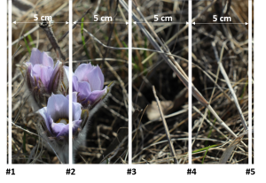
- Use tape to make 5 transects that are equally spaced and parallel to one another (see Figure 1 for an example).
- For each habitat colour, measure the transect length (i.e., distance) that it covers (mm) and record in Table 2 (sample table provided below). For colours that are not the same as the phenotype of the dots, simply add all measurements to the “other” column.
- For each transect, add up the lengths for the transect – this should be similar for all transects. If not, remeasure any that are not similar to the length shown on the tape measure.
- Calculate the mean cover values and then calculate the proportion of the habitat that is covered by each colour (i.e., divide the mean length of each colour by the transect length). Ask for assistance as needed.

Figure 1. Example of 5 equally spaced transects (white lines are the transects)
| Sample Table 2. Data table for habitat colour features. | |||||||||
| Habitat colour | Black | Orange | White | … | … | … | … | Other | Total transect length (mm) |
| Transect 1 | |||||||||
| Transect 2 | |||||||||
| Transect 3 | |||||||||
| Transect 4 | |||||||||
| Transect 5 | |||||||||
| Mean Cover (mm) | |||||||||
| Proportion of habitat | |||||||||

